BRIN Indexes – Operation
PostgreSQL 9.5 released in january 2016 brings a new kind of index: BRIN indexes for Bloc Range INdex. They are recommanded when tables are very big and correlated with their physical location. I decided to devote a series of articles on these indexes:
- BRIN Indexes - Overview
- BRIN Indexes - Operation
- BRIN Indexes - Correlation
- BRIN Indexes - Performances
In this second article we will see how BRIN indexes works.
Operation
Index will contain the minimal and maximal value 1 of an attribute for a range of blocks.
Range’s size is 128 blocks (128 x 8KB => 1MB)
Take an example, a 100 000 lines table composed by a column “id” incremented by 1. Basically, the table will be stored like this (one bloc can contain several tuples) :
| Bloc | id |
|---|---|
| 0 | 1 |
| 0 | 2 |
| … | … |
| 1 | 227 |
| … | … |
| 128 | 28929 |
| … | … |
| 255 | 57856 |
| 256 | 57857 |
| … | … |
1CREATE TABLE t1 (c1) AS (SELECT * FROM generate_series(1,100000));
2SELECT ctid,c1 from t1;
If we search for value between 28929 et 57856, PostgreSQL will have to read the whole table. It do not know it is not necessary to read before block 128 and after block 255.
First reaction will be to create a B-tree index. Without going into details, this kind of index allows a more efficient read of the table. It will contain each location of each value of the table.
Basically, omitting tree view, the index would contain:
| id | Location |
|---|---|
| 1 | 0 |
| 2 | 0 |
| … | |
| 227 | 1 |
| … | … |
| 57857 | 256 |
Intuitively we can already deduce that if our table is large, the index will also be large.
BRIN index will contain theses rows:
| Range (128 blocks) | min | max | allnulls | hasnulls |
|---|---|---|---|---|
| 1 | 1 | 28928 | false | false |
| 2 | 28929 | 57856 | false | false |
| 3 | 57857 | 86784 | false | false |
| 4 | 86785 | 115712 | false | false |
1create index ON t1 using brin(c1) ;
2create extension pageinspect;
3SELECT * FROM brin_page_items(get_raw_page('t1_c1_idx', 2), 't1_c1_idx');
So looking for the values between 28929 and 57856 Postgres knows that it will have to go through blocks 128 to 255.
Comparing to a B-tree, we could represent in 4 rows what would have taken more than 100 000 rows in a B-tree. Or course, reality is much more complex, however, this simplification already provides an overview of the compactness of this index.
Influence of the size of the range
Default range size is 128 blocks, which corresponds to 1MB (1 block is 8KB). We will test with differents range size thanks to the pages_per_range option.
Let’s take a bigger data set, with 100 million lines:
1CREATE TABLE brin_large (c1 INT);
2INSERT INTO brin_large SELECT * FROM generate_series(1,100000000);
Table size is arround 3.5GB:
1\dt+ brin_large
2                       List OF relations
3 Schema |    Name    | TYPE  |  Owner   |  SIZE   | Description
4--------+------------+-------+----------+---------+-------------
5 public | brin_large | TABLE | postgres | 3458 MB |
Enable psql “\timing” option to measure index creation time. Let’s start with BRIN with a different pages_per_range:
1CREATE INDEX brin_large_brin_idx ON brin_large USING brin (c1);
2CREATE INDEX brin_large_brin_idx_8 ON brin_large USING brin (c1) WITH (pages_per_range = 8);
3CREATE INDEX brin_large_brin_idx_16 ON brin_large USING brin (c1) WITH (pages_per_range = 16);
4CREATE INDEX brin_large_brin_idx_32 ON brin_large USING brin (c1) WITH (pages_per_range = 32);
5CREATE INDEX brin_large_brin_idx_64 ON brin_large USING brin (c1) WITH (pages_per_range = 64);
Also create a b-tree:
1CREATE INDEX brin_large_btree_idx ON brin_large USING btree (c1);
Compare size:
 1\di+ brin_large*
 2                                    List OF relations
 3 Schema |          Name          | TYPE  |  Owner   |   TABLE    |  SIZE   | Description
 4--------+------------------------+-------+----------+------------+---------+-------------
 5 public | brin_large_brin_idx    | INDEX | postgres | brin_large | 128 kB  |
 6 public | brin_large_brin_idx_16 | INDEX | postgres | brin_large | 744 kB  |
 7 public | brin_large_brin_idx_32 | INDEX | postgres | brin_large | 392 kB  |
 8 public | brin_large_brin_idx_64 | INDEX | postgres | brin_large | 216 kB  |
 9 public | brin_large_brin_idx_8  | INDEX | postgres | brin_large | 1448 kB |
10 public | brin_large_btree_idx   | INDEX | postgres | brin_large | 2142 MB |
Here are the results on the index creation times and their sizes:
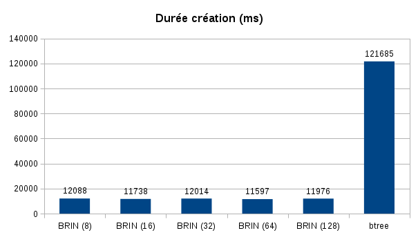
Index creation is faster. The gain is arround x10 between two indexes type. Tested with a pretty basic configuration (laptop, mechanical HDD). I advise you to conduct your own tests with your material.
FYI I used a maintenance_work_mem at 1GB. Despite this high value, sort did not fit in RAM so it generates temps files for B-tree index.
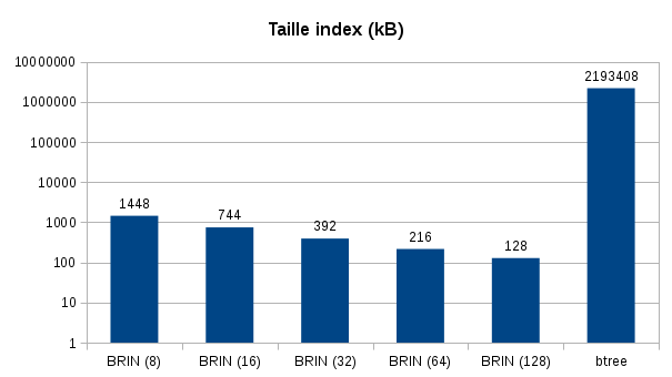
For index size, difference is much more important, I used a logarithmic scale to represent gap. BRIN with a default pages_per_range is 128KB while B-tree is more than 2GB!
What about queries?
Let’s try this query which retrieves the values between 10 and 2000. To study in detail what Postgres does we will use EXPLAIN with the options (ANALYZE, VERBOSE, BUFFERS).
Finally, to facilitate the analysis we will use a smaller data set:
1CREATE TABLE brin_demo (c1 INT);
2INSERT INTO brin_demo SELECT * FROM generate_series(1,100000);
 1EXPLAIN (ANALYZE,BUFFERS,VERBOSE) SELECT c1 FROM brin_demo WHERE c1> 1 AND c1<2000;
 2 QUERY PLAN
 3-------------------------------------------------------------------------------------------------------------------
 4 Seq Scan on public.brin_demo (cost=0.00..2137.47 rows=565 width=4) (actual time=0.010..11.311 rows=1998 loops=1)
 5 Output: c1
 6 Filter: ((brin_demo.c1 > 1) AND (brin_demo.c1 < 2000))
 7 Rows Removed by Filter: 98002
 8 Buffers: shared hit=443
 9 Planning time: 0.044 ms
10 Execution time: 11.412 ms
Without index Postgres read the entire table (seq scan) and reads 443 blocks.
The same query with a BRIN index:
 1CREATE INDEX brin_demo_brin_idx ON brin_demo USING brin (c1);
 2EXPLAIN (ANALYZE,BUFFERS,VERBOSE) SELECT c1 FROM brin_demo WHERE c1> 1 AND c1<2000;
 3 QUERY PLAN
 4---------------------------------------------------------------------------------------------------------------------------------
 5 Bitmap Heap Scan on public.brin_demo (cost=17.12..488.71 rows=500 width=4) (actual time=0.034..3.483 rows=1998 loops=1)
 6 Output: c1
 7 Recheck Cond: ((brin_demo.c1 > 1) AND (brin_demo.c1 < 2000))
 8 Rows Removed by Index Recheck: 26930
 9 Heap Blocks: lossy=128
10 Buffers: shared hit=130
11 -> Bitmap Index Scan on brin_demo_brin_idx (cost=0.00..17.00 rows=500 width=0) (actual time=0.022..0.022 rows=1280 loops=1)
12 Index Cond: ((brin_demo.c1 > 1) AND (brin_demo.c1 < 2000))
13 Buffers: shared hit=2
14 Planning time: 0.074 ms
15 Execution time: 3.623 ms
Postgres reads 2 index blocks then 128 blocks from table.
Let’s try with a smaller pages_per_range, for example:
 1CREATE INDEX brin_demo_brin_idx_16 ON brin_demo USING brin (c1) WITH (pages_per_range = 16);
 2EXPLAIN (ANALYZE,BUFFERS,VERBOSE) SELECT c1 FROM brin_demo WHERE c1> 10 AND c1<2000;
 3 QUERY PLAN
 4-----------------------------------------------------------------------------------------------------------------------------------
 5 Bitmap Heap Scan on public.brin_demo (cost=17.12..488.71 rows=500 width=4) (actual time=0.053..0.727 rows=1989 loops=1)
 6 Output: c1
 7 Recheck Cond: ((brin_demo.c1 > 10) AND (brin_demo.c1 < 2000))
 8 Rows Removed by Index Recheck: 1627
 9 Heap Blocks: lossy=16
10 Buffers: shared hit=18
11 -> Bitmap Index Scan on brin_demo_brin_idx_16 (cost=0.00..17.00 rows=500 width=0) (actual time=0.033..0.033 rows=160 loops=1)
12 Index Cond: ((brin_demo.c1 > 10) AND (brin_demo.c1 < 2000))
13 Buffers: shared hit=2
14 Planning time: 0.114 ms
15 Execution time: 0.852 ms
Again Postgres reads 2 blocks from the index, however it will only read 16 blocks from the table.
An index with a smaller pages_per_range will be more selective and will allow you to read fewer blocks.
Use the pageinspect extension to observe the contents of the indexes:
 1CREATE extension pageinspect;
 2SELECT * FROM brin_page_items(get_raw_page('brin_demo_brin_idx_16', 2),'brin_demo_brin_idx_16');
 3 itemoffset | blknum | attnum | allnulls | hasnulls | placeholder | value
 4------------+--------+--------+----------+----------+-------------+-------------------
 5 1 | 0 | 1 | f | f | f | {1 .. 3616}
 6 2 | 16 | 1 | f | f | f | {3617 .. 7232}
 7 3 | 32 | 1 | f | f | f | {7233 .. 10848}
 8 4 | 48 | 1 | f | f | f | {10849 .. 14464}
 9 5 | 64 | 1 | f | f | f | {14465 .. 18080}
10 6 | 80 | 1 | f | f | f | {18081 .. 21696}
11 7 | 96 | 1 | f | f | f | {21697 .. 25312}
12 8 | 112 | 1 | f | f | f | {25313 .. 28928}
13 9 | 128 | 1 | f | f | f | {28929 .. 32544}
14 10 | 144 | 1 | f | f | f | {32545 .. 36160}
15 11 | 160 | 1 | f | f | f | {36161 .. 39776}
16 12 | 176 | 1 | f | f | f | {39777 .. 43392}
17 13 | 192 | 1 | f | f | f | {43393 .. 47008}
18 14 | 208 | 1 | f | f | f | {47009 .. 50624}
19 15 | 224 | 1 | f | f | f | {50625 .. 54240}
20 16 | 240 | 1 | f | f | f | {54241 .. 57856}
21 17 | 256 | 1 | f | f | f | {57857 .. 61472}
22 18 | 272 | 1 | f | f | f | {61473 .. 65088}
23 19 | 288 | 1 | f | f | f | {65089 .. 68704}
24 20 | 304 | 1 | f | f | f | {68705 .. 72320}
25 21 | 320 | 1 | f | f | f | {72321 .. 75936}
26 22 | 336 | 1 | f | f | f | {75937 .. 79552}
27 23 | 352 | 1 | f | f | f | {79553 .. 83168}
28 24 | 368 | 1 | f | f | f | {83169 .. 86784}
29 25 | 384 | 1 | f | f | f | {86785 .. 90400}
30 26 | 400 | 1 | f | f | f | {90401 .. 94016}
31 27 | 416 | 1 | f | f | f | {94017 .. 97632}
32 28 | 432 | 1 | f | f | f | {97633 .. 100000}
33(28 lignes)
34
35SELECT * FROM brin_page_items(get_raw_page('brin_demo_brin_idx', 2),'brin_demo_brin_idx');
36 itemoffset | blknum | attnum | allnulls | hasnulls | placeholder | value
37------------+--------+--------+----------+----------+-------------+-------------------
38 1 | 0 | 1 | f | f | f | {1 .. 28928}
39 2 | 128 | 1 | f | f | f | {28929 .. 57856}
40 3 | 256 | 1 | f | f | f | {57857 .. 86784}
41 4 | 384 | 1 | f | f | f | {86785 .. 100000}
42(4 lignes)
With the index brin_demo_brin_idx_16 we note that the values we are interested in are present in the first set of blocks (0 to 15). On the other hand, with the index brin_demo_brin_idx, this one is less selective. The values that interest us are included in blocks 0 to 127 which explains why there are more blocks read in the first example.
-
Index also contains two Booleans that indicate whether the set contains nulls (hasnulls) or contains only nulls (allnulls) ↩︎

For seven years, I held various positions as a systems and network engineer. And it was in 2013 that I first started working with PostgreSQL. I held positions as a consultant, trainer, and also production DBA (Doctolib, Peopledoc).
This blog is a place where I share my findings, knowledge and talks.