BRIN Indexes – Performances
PostgreSQL 9.5 released in january 2016 brings a new kind of index: BRIN indexes for Bloc Range INdex. They are recommanded when tables are very big and correlated with their physical location. I decided to devote a series of articles on these indexes:
- BRIN Indexes - Overview
- BRIN Indexes - Operation
- BRIN Indexes - Correlation
- BRIN Indexes - Performances
This article is the last of the series, it will be dedicated to performances (maintenance, reading, insertion …)
Performances
Previous articles have discussed the operation and specificities of the BRIN indexes. This article will be more about performance. Previous examples were done on small dataset. Now we will see what can bring these indexes on a larger volume.
The tests were performed on a laptop, transaction logs, table and indexes are stored on a mechanical disk. The results will be different depending on the equipment used. These figures are purely indicative and serve mainly to give an idea.
Example
At first it is necessary to create a table with a large dataset.
For example: a measurement system with 100 probes and a measurement every second. We will therefore obtain 100*365*24*3600 measures => a little more than 3 billion lines.
 1-- Using a function to generate random text.
 2-- From : http://stackoverflow.com/questions/3970795/how-do-you-create-a-random-string-in-postgresql
 3
 4CREATE OR REPLACE FUNCTION random_string(LENGTH INTEGER) RETURNS text AS
 5$$
 6DECLARE
 7  chars text[] := '{0,1,2,3,4,5,6,7,8,9,A,B,C,D,E,F,G,H,I,J,K,L,M,N,O,P,Q,R,S,T,U,V,W,X,Y,Z,a,b,c,d,e,f,g,h,i,j,k,l,m,n,o,p,q,r,s,t,u,v,w,x,y,z}';
 8  RESULT text := '';
 9  i INTEGER := 0;
10BEGIN
11  IF LENGTH < 0 THEN
12    raise exception 'Given length cannot be less than 0';
13  END IF;
14  FOR i IN 1..LENGTH loop
15    RESULT := RESULT || chars[1+random()*(array_length(chars, 1)-1)];
16  END loop;
17  RETURN RESULT;
18END;
19$$ LANGUAGE plpgsql;
20-- Creation de la table contenant les sondes
21CREATE TABLE probe (id serial PRIMARY KEY, name text);
22INSERT INTO probe (name ) SELECT random_string(5) FROM generate_series(1,100);
23
24CREATE TABLE data AS
25WITH generation AS (
26SELECT '2015-01-01'::TIMESTAMP + i * INTERVAL '1 second' AS date_metric,sonde::text,random() AS metric
27FROM generate_series(0, 3600*24*365) i,
28LATERAL (SELECT name FROM probe) sonde)
29SELECT * FROM generation;
The resulting table is a little more than 150GB, so it does not fit in the RAM of the machine hosting the instance and even less in the shared buffers.
Maintenance
We create many indexes to compare their size:
1CREATE INDEX metro_btree_idx ON data USING btree (date_metric);
2CREATE INDEX metro_brin_idx_8 ON data USING brin (date_metric) WITH (pages_per_range = 8);
3CREATE INDEX metro_brin_idx_16 ON data USING brin (date_metric) WITH (pages_per_range = 16);
4CREATE INDEX metro_brin_idx_32 ON data USING brin (date_metric) WITH (pages_per_range = 32);
5CREATE INDEX metro_brin_idx_64 ON data USING brin (date_metric) WITH (pages_per_range = 64);
6CREATE INDEX metro_brin_idx_128 ON data USING brin (date_metric);
7CREATE INDEX metro_brin_idx_256 ON data USING brin (date_metric) WITH (pages_per_range = 256);
Here are the results obtained for the duration of creation of indexes and their sizes:
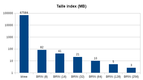
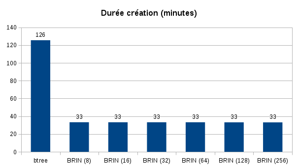
Index creation was 4 times faster for BRIN indexes. It is possible that their creation would have been faster with more efficient storage.
The size of the indexes is also striking, the b-tree index is 66 GB whereas the index BRIN with the default pages_per_range is only 5 MB.
We can immediately see the gain on the space used and the speed of creation of the indexes. Maintenance operations (REINDEX) will be greatly facilitated.
Read performance
We will perform several tests, the idea is to try to highlight the differences in behavior between the BRIN and b-tree indexes.
The query used will be very simple:
1EXPLAIN (ANALYSE,BUFFERS,VERBOSE) SELECT date_metric,sonde,metric FROM DATA WHERE date_metric = 'xxx';
To get a result with few lines:
1WHERE date_metric = '2015-05-01 00:00:00'::TIMESTAMP
To obtain more results we will take an interval with:
1WHERE date_metric BETWEEN 'xxx'::TIMESTAMP AND 'xxx'::TIMESTAMP;
Here are the results obtained:
| Rows |
|---|
| Duration |
| 100 |
| 267 million |
| 777 million |
| 1.3 billion |
To compare the volume of data read and the execution time we can disable indexes in a transaction:
1BEGIN;
2DROP index ...;
3explain (analyse,verbose,buffers) SELECT ...
4rollback;
For the first test, postgres chooses b-tree index. By deleting b-tree index, he chooses BRIN index.
For tests 2 and 3, postgres chooses BRIN index, by removing BRIN index it chooses b-tree index.
For the last test I added other measures. Indeed, by removing the index BRIN postgres will perform a seqscan (read entire table). To obtain the same comparisons as the previous results, I deleted the BRIN index and disabled the sequential runs (set enable_seqscan to 'off';)
Overall we can see a gain of 30-40% in cases where many rows are fetched. postgres reads fewer blocks when using the BRIN indexes, b-tree index being large, its readings are expensive.
On the other hand, b-tree index is particularly powerful when the query is very selective and few results are returned. Indeed, using a BRIN index, postgres starts by reading the entire index. Then it will read a set of blocks that contain the desired value, some not containing any results. These additional readings are felt on the execution time of the request.
Insertion performance
Since the BRIN indexes are smaller and their creation time shorter, one wonders what happens to the extra cost of this index when inserting data. For that we will create a table and measure the insertion of 10 million lines according to the indexes already present on the table. In order to target the extra cost due to index updates, the table is unlogged, in order to avoid extra WAL writes. Autovacuum is also disabled.
 1CREATE UNLOGGED TABLE brin_demo_2 (c1 INT);
 2INSERT INTO brin_demo_2 SELECT * FROM generate_series(1,10000000);
 3TRUNCATE brin_demo_2;
 4
 5CREATE INDEX brin_demo_2_brin_idx ON brin_demo_2 USING brin (c1);
 6INSERT INTO brin_demo_2 SELECT * FROM generate_series(1,10000000);
 7DROP INDEX brin_demo_2_brin_idx;
 8TRUNCATE brin_demo_2;
 9
10CREATE INDEX brin_demo_2_brin_idx ON brin_demo_2 USING brin (c1) WITH (pages_per_range = 256);
11INSERT INTO brin_demo_2 SELECT * FROM generate_series(1,10000000);
12DROP INDEX brin_demo_2_brin_idx;
13TRUNCATE brin_demo_2;
14...
Here are the results obtained:
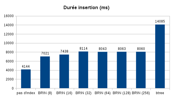
However, we can see that it is cheaper to insert data in a table with a BRIN index than with a b-tree index. We also note that there is no significant difference between the different types of BRIN indexes.
Conclusion
This series of articles made it possible to present the principles of the BRIN indexes. then their operation through simple examples.
Then we saw the importance of correlation to fully exploit these indexes. Finally, we tried to measure the gain that could bring this index on multiple aspects (maintenance, performance in reading and insertion).
Describing the operation of an index by simplifying its representation is a complicated exercise. Presenting numbers is also tricky so they can depend on the context. I made the effort to detail how I got them so that everyone could reproduce their own tests. The idea is to give an overview of the use cases of this type of index.
Overall it should be remembered that BRIN indexes are useful for large tables and where the correlation with the location of the data is important. They will be slower than the b-tree indexes when the search requires running a few blocks. They will be a little faster than b-tree indexes in situations where postgres has to read a lot of blocks (fewer blocks to read in the index).
The study of this index opens other ways for reflection. Like taking into account the correlation in the calculation of the cost. I had also thought about the possibility of using an index to create another index.
In the example with the large table (150GB). If you want to create a partial index on the previous month, the engine will browse the entire table to create index. One could consider creating the index b-tree using the index BRIN to browse only lines corresponding to the previous least.

For seven years, I held various positions as a systems and network engineer. And it was in 2013 that I first started working with PostgreSQL. I held positions as a consultant, trainer, and also production DBA (Doctolib, Peopledoc).
This blog is a place where I share my findings, knowledge and talks.